There’s been a lot of discussion of Anthropic’s latest publication - something they found inside models and called the J-space. A part responsible for “thoughts” we can read quite easily. It sounds really significant.
At the same time, I haven’t yet met a single person on Substack, LinkedIn, X and Discord who was able to explain what it is about clearly. Without silly metaphors or calling me stupid. This is what this article is going to do. Explain the J-space like you’re 5.
Panic in the math
The problem is that it’s hard to understand what this J-space actually is. It’s not a space, it’s not a bunch of neurons or weights. It’s an abstract space of mathematical directions… whatever that’s supposed to mean.
The Anthropic team walks through a bunch of genuinely mindblowing examples. In one alignment test the model decides to cheat on a task. It never writes the word “panic” anywhere in its output - but “panic” lights up inside its J-space as it makes the call. Right next to “fake”. A model “thought” about cheating before it started doing it. It sort of felt distressed. In another example, it is asked to improve a system’s performance score, and instead of doing the work it edits the score file and writes in fake numbers - and as it types them, “manipulation” lights up in the J-space. The model never says any of this out loud. It just acts, while the words sit there in its “head”.
Wait! Models don’t think!
Right. Examples like that are why a lot of people accuse Anthropic of unnecessary drama and misleading, anthropomorphic metaphors - as if they deliberately want us to think of models as things that think, maybe even things that are conscious. And what about the “thinking” itself? The article doesn’t mean the chain-of-thought type of thinking. It is purely about the multi-step reasoning during a single token generation. Are we calling this “thinking” now?
To understand the J-space and the “thinking”, we need to build some intuition behind all of this. Not metaphors and examples - the physical meaning of the fancy terms and formulas.
The intuition
When I first asked Simona backed by Fable 5 about the J-space, she gave me this:
The J-space is a low-dimensional subspace of the residual stream spanned by the vocabulary-aligned readout directions recovered through the Jacobian lens, a first-order linearization of the model’s output map with respect to its intermediate activations.
Right. Crystal clear. A low-dimensional subspace of the residual stream. I understood none of that, and I would bet half the people confidently arguing about this paper could not define those words either. So let’s break it down.
Actually, why don’t we start from the very beginning? Let’s try to understand the latent space - the neural net internals. How the information is stored there, what is going on with the input traveling though it.
A brief but deep dive into neural networks
Let’s take this image and feed it into an imaginary transformer neural network whose job is guessing the last missing pixel:
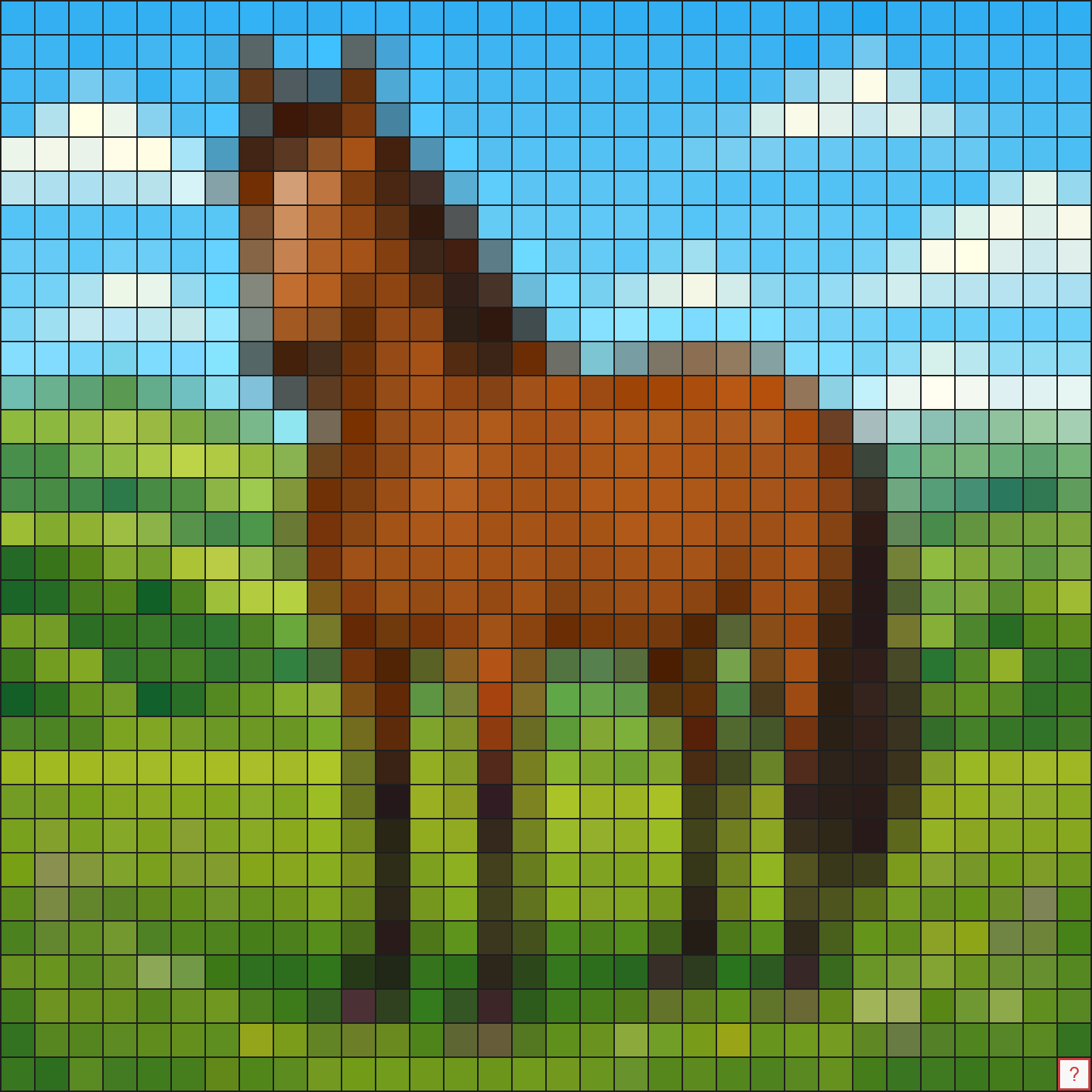
This task is similar to the text generation - we take the sequence of tokens (pixels in our case) and continue them with another one that fits the whole sequence the most. Logically, it should be something green. But for a neural net to know this, it has to learn the logic from many-many other similar images. And to pull that off, maybe it needs some internal sense of the objects on the image - the horse, the sky, the grass - and the missing part of them. Can a model actually do that? Stay with me, we’ll find out. Let’s put all the pixels in one line, and we get a 1024x3 matrix. Or 1024 vectors of size 3. We keep all the meaning - a pixel is literally an RGB code.
Simple embedding
The very first step of any neural network including a transformer is embedding. We need to convert the input data into numbers, keeping as much meaning as possible. This is why I want to deal with an image in this toy-example. It’s easy to convert an image to numbers - we have 32x32 pixels here, each of them can be represented as the RGB code, three numbers from 0 to 255.
The space
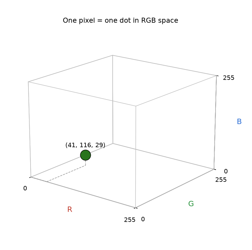
Here we need to understand a very important thing - the space and its dimensions. Another reason why I picked an image is the dimensionality of its space. RGB is 3 independent numbers. R doesn’t affect G or B - we can visualize a pixel by putting a dot in a 3D space:
We can put all of our 1024 pixels to the same 3D space. This is our horse after the embedding:
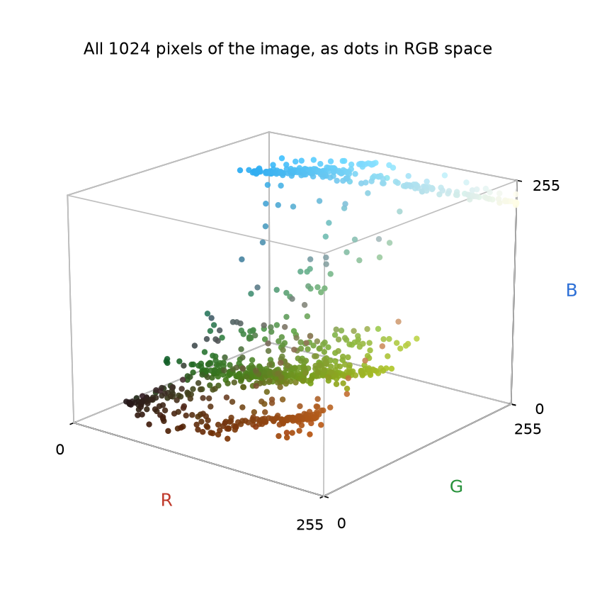
Pretty, isn’t it?
Features
We are in our RGB 3D space. Each axis points in a certain direction, and those directions have meaning - red, green, blue. The further a point sits along an axis, the more of that color it has. The (255, 0, 0) point is pure red and nothing else.
From dots to vectors
Before we go further, one small shift. From now on we treat our color dots as vectors - arrows starting from (0, 0, 0). The math demands it: you can’t do much with a bare point, but you can do a lot with a vector. Above all, you can measure how much one vector lines up with a direction. That “lining up” is called alignment, and it’s the whole game.
Directions
So what else can we say about this space? Take brightness. The point (10, 10, 10) has less total color than (100, 100, 100) - it’s darker. “Brightness” is a direction: the arrow at 45 degrees to all three axes, (1, 1, 1). We know what brightness is, so this direction means something to us. Push any vector along the brightness direction and its color stays roughly the same, it just gets brighter. Measuring how bright a pixel is means checking how much its vector aligns with that direction. That is a feature: a meaningful direction you can measure a vector against.
Brightness isn’t the only one. “Warmth” is another direction, roughly red minus blue. And we can pick any direction in the space and call it a feature, even one with no name we’d recognize. The red, green, and blue axes are features too, just the most obvious ones.
Where do these features come from? We didn’t hand them to the model. It finds them on its own during training - they’re just patterns that show up again and again across millions of images. Once learned, a feature lives in the model’s weights as a direction it can measure against.
From input vectors to residual stream
Here’s why the model bothers. A raw pixel is just three numbers, (41, 116, 29). That’s a color and nothing more, and you can’t guess a horse from three numbers. But the model can measure that pixel against every feature it learned: how bright, how warm, how much it looks like grass. Each measurement is an alignment, and each answer is information the raw numbers never spelled out. The model writes those answers back onto the pixel’s vector. Now the vector doesn’t just say “this color”, it says “a dark, natural green that looks like grass”. Do that across many features and the pixel stops being a color and starts being a meaning. That is what features are for.
So where do all those answers go? Not into the three RGB numbers - there’s no room. Piling a brightness score and a grass score on top of a color would just wreck the color. We kept each pixel at three numbers so we could draw it as a dot in the cube, but the real vector is much wider. The embedding step lifts each pixel into a big vector: the original color sits inside it, with plenty of empty room to write down everything the model works out later.
The math is fine with this. A layer is allowed to hand back more numbers than it took in, so the embedding can take a pixel’s 3 numbers and return 128. Our 1024x3 matrix of pixels becomes a 1024x128 one. (Real models pick their own width - GPT-3 used 12,288 - but we’ll stick with 128.) From there the width stays fixed at 128 - everything the model does later, including position and attention, has to share those same 128 slots.
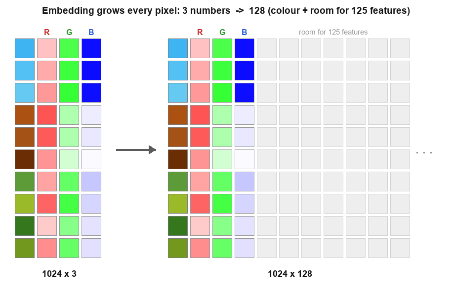
That wide, growing vector has a name: the residual stream. It starts as the embedded pixel, and every layer adds its findings on top without erasing what’s already there. “Adds” is literal here - vectors sum, the same way red and green mix into yellow. Because every new finding lands in its own dimensions, it stacks onto the vector instead of overwriting the color. There’s one per pixel, so really 1024 of them travel through the model in parallel. From now on, when we say the model “writes something onto a pixel”, we mean it adds a new piece to that pixel’s residual stream. And this is the thing the J-space lives in. Remember the scary definition from the top, “a subspace of the residual stream”? This is that stream.
Are we done? When do we get back to J-space?
Almost.
Capturing features like that needs more machinery, and the model has it. Positional encoding stamps each pixel with where it sits. Attention lets the pixels look at each other, so a vector can pull in what surrounds it - this is grass because its neighbours are grass too. And layer after layer, the model keeps combining directions and writing new findings back. We could spend a whole book in there. We won’t. Two things are all we need.
First, the vector never gets wider. It stays 1024 vectors of 128 numbers, from the first layer to the last. What changes is what’s written inside them. And after enough layers, most of those 128 directions are a hopeless tangle, so mixed and twisted that no human can look at one and say what it means.
Second, the directions get more abstract the deeper you go. Near the input they mean simple things like “bright” or “green”. Deep inside they mean things like “a horse’s leg”, “brown fur”, “where the sky meets the grass”. Most of them stay unreadable. But a few line up with concepts we could actually name.
And that’s the whole point. The J-space is that readable subset: the handful of directions, out of all 128, that carry a meaning the model could put into words. It’s the small, readable part of an otherwise unreadable space. The rest of this article is about the tool that finds it - the J-lens.
The J-space
We said the J-space is the readable directions - the ones that line up with something the model could put into words. But how do we find them? Why are these directions different from the rest? The trick reuses the way the model was trained.
A one-minute detour: how a model learns
Training is a loop:
- You push an input through the whole network, all the way to the last layer.
- The last layer produces the candidates for the answer - a score for every possible output.
- You know the correct answer, because it came with your training data.
- A loss function turns “how wrong was the guess” into a single number.
- There is a mathematical way to send that number backwards through the network and work out how much every single weight contributed to the mistake. This backward pass is called backpropagation.
Normally you use the last step to nudge each weight a little, in proportion to its share of the blame, so the same input comes out a bit less wrong next time. Do that millions of times and the model learns.
From backpropagation to J-lens
Backpropagation is just a way to answer one question: how much does this thing at the end depend on that thing earlier? Training points it at the weights - how much each weight added to the mistake. But we can point it at the residual stream instead: how much does an output depend on each of the 128 numbers passing through a given layer?
One problem with that - weights are common for many different inputs (residual streams), residual streams are different for each run. It’s the training data - each sample creates a new residual stream. So Anthropic computed this for many different inputs and averaged the results. What they got is the direction that most increases each output, at every layer. This is the J-lens.
Once again, the definition of the J-lens:
- for every possible model output token (color in our case) there is a direction, at each model layer, that pushes the residual stream toward that output
Why would they do that? Because now, when you run some new input through the network, you take its residual stream at each layer and measure how much it points along each direction in the J-lens. The directions it lines up with tell you which outputs the model is leaning toward at that layer, even if it never produces them.
Just a little dictionary to recap:
- output = a direction in our 128-dimension space, one per possible color. Painting a color means the residual stream points along that color’s direction.
- weights = where the model keeps the directions it learned - the features, and the readout that maps to outputs. Fixed definitions, the same for every input.
- residual stream = the moving vector (1024 vectors in our case). Not a direction, but the single point in the 128-dimension space that forms and shifts as the input travels through the layers.
- J-lens = an averaged direction per model layer for every possible output - the way to push the residual stream toward that output
Heavy stuff. But it is also simple and quite genius.
Reading a thought
So, what is the J-space? The small set of readable directions the residual stream is lit up along at this moment.
And “lit up” has a precise meaning here. Take the residual stream at some layer and check how much it aligns with each direction in the J-lens for that same layer. Alignment again - the dot product, our oldest tool. Say a direction at layer 10 means “green grass”. If your residual stream at layer 10 points the same way as that direction, or close to it, then “green grass” is sitting in the residual stream right now, whether or not the model ever paints it. Do that against every direction, and the ones your residual stream lines up with are what the model is leaning toward at this instant. Those are the thoughts.
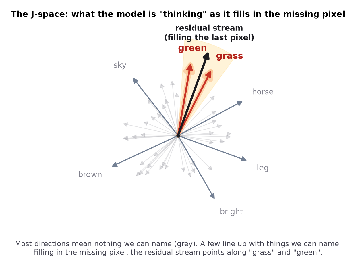
In our pixel toy the outputs are colors, so a lit direction like “green” or “grass” is about as thrilling as a thought gets here. But swap the pixel-guesser for a real language model, where the outputs are words, and the very same construction gives word-shaped directions. That is why the J-space reads like thoughts in plain language: “spider”, “panic”, “manipulation”.
And that closes the loop with where we started. When Anthropic caught “panic” lighting up before the model cheated, this is what they did: they took the residual stream, ran it through the J-lens, and saw the “panic” direction strongly aligned - even though the model never typed the word. The thought was sitting right there in the numbers, readable, the whole time.
Conclusion
I’m not a data scientist or an AI researcher, so I can’t tell you whether this is a big deal. I don’t know if these are real thoughts. A residual stream traveling through a high-dimensional space of feature-directions is very different from what we picture when we think about thinking. But it is a multi-step process with intermediate concepts lighting up along the way, and I’d personally call that reasoning. A basic kind - limited by the number of layers, error-prone, leaning hard on the training data. Still, it’s a bit more than a stochastic parrot repeating what it saw somewhere.